Financial Institutions Survey Analysis Part 1

Financial Institutions Survey Analysis

 1. Data    

Survey data consist of the 99 observations and 73 variables.

This study focuses on assessing the internal control systems and their impact on the operational 

efficiency of financial institutions in Nigeria.

2. Clean data, convert data

3. Data summary

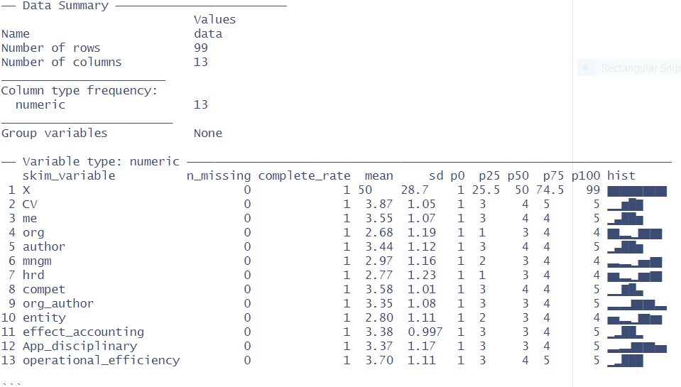
4. Plot distribution

5.Multi linear regression model statistics

Use the multi linear model statistics

In this case will use operational efficiency as dependent variable, and the independent 

variables, as example:

Variables need to be abbreviated to make it easier to create a model.

CV:  "section_a_control_environment_the_following_statements_pertain_to_how_the_control_environment_influences_the_financial_performance_of_the_microfinance_bank_please_rate_each_statement_according_to_your_understanding_by_selecting_the_appropriate_option_communication_and_enforcement_of_integrity_and_ethical_values_within_our_microfinance_bank_are_adequate",

me:  "our_microfinance_bank_management_is_dedicated_to_ensuring_employee_competence_in_financial_matters",                                                                                                                                                        org:  "the_managements_philosophy_and_operating_style_promote_the_microfinance_banks_growth_while_maintaining_adherence_to_rules_and_regulations",                                                                                  author:  "the_microfinance_bank_s_organizational_structure_has_clear_lines_for_reporting_and_decision_making_hierarchies",                                                                                                                                              mngm:  "our_microfinance_banks_management_appropriately_assigns_authority_and_responsibility_to_qualified_individuals",                                                                                                                                              hrd:  "we_have_well_designed_human_resource_policies_that_are_easy_to_implement_and_practice_within_our_microfinance_bank",                                                                                                                            compet:  "the_microfinance_bank_is_committed_to_ensuring_competence_in_job_specific_requirements_and_the_translation_of_ those_requirements_into_necessary_knowledge_and_skills",                                                                                                                                                                                                   org_author:  "the_organization_assigns_authority_and_responsibility_to_foster_accountability_and_control",                                                                                                                                                                                    entity:  "the_entity_assigns_authority_and_responsibility_to_provide_a_basis_for_accountability_and_control",                                                                                                                                                                      effect_accounting:  "the_microfinance_bank_has_an_effective_accounting_and_financial_management_system_in_place",                                                                                                                                                                          App_disciplinary:  "appropriate_disciplinary_actions_are_taken_when_employees_fail_to_comply_with_policies_procedures_or_behavioral_standards", 

 #---Dependent variable

operational efficiency: "section_f_operational_efficiency_please_indicate_your_level_of_agreement_with_the_following_statements_regarding_the_performance_of_your_organization_microfinance_bank_s_financial_statements_aim_to_provide_a_comprehensive_overview_of_the_organization_s_performance_and_position_at_a_specific_point_in_time"

 6.1 Control environment 

To assess the effect of the control environment on the operational efficiency of financial institutions.

We can see from the table of the multi linier statistics model regression:

#---

# Coefficients:

#                                               Estimate Std. Error t value Pr(>|t|)    

# (Intercept)                    2.7653917  0.7311077   3.782 0.000286 ***

# X                                 -0.0011205  0.0040307  -0.278 0.781693    

# CV                                0.0008834  0.1259978   0.007 0.994422    

# me                               -0.0411602  0.1206962  -0.341 0.733918    

# org                               -0.1852678  0.1055421  -1.755 0.082753 .  

# author                          -0.1898709  0.1128253  -1.683 0.096027 .  

# mngm                           0.0548492  0.1015565   0.540 0.590534    

# hrd                                0.2139908  0.0952287   2.247 0.027192 *  

# compet                          0.2940369  0.1283810   2.290 0.024448 *  

# org_author                   -0.0739613  0.1143838  -0.647 0.519609    

# entity                           -0.0863652  0.1106345  -0.781 0.437160    

# effect_accounting          0.2746892  0.1316306   2.087 0.039865 *  

#  App_disciplinary          0.0099777  0.1087175   0.092 0.927089    

#---

#  Signif. codes:  0 ‘***’ 0.001 ‘**’ 0.01 ‘*’ 0.05 ‘.’ 0.1 ‘ ’ 1

# Residual standard error: 1.079 on 86 degrees of freedom

# Multiple R-squared:  0.1715, Adjusted R-squared:  0.05595 

# F-statistic: 1.484 on 12 and 86 DF,  p-value: 0.1459

The three variables hrd(0.027192 *),compet( 0.024448 *) and effect_accounting(0.039865 *) have weak effects on the operational efficiency of financial institutions. 

The CV variable(0.994422) have no statistical influence to operational efficiency of financial.

Based on the  F-statistic of the model 1.484 and the corresponding p-value: 0.1459. This indicates that the overall model is not statistically significant because the p-value: 0.1459 is greater than 0.05.

6.2. Risk assessment

#----

# Coefficients:

#                                            Estimate Std. Error t value Pr(>|t|)    

# (Intercept)                   2.334e+00  5.144e-01   4.536 1.69e-05 ***

#                                      6.325e-05  3.532e-03   0.018   0.9857    

# risk_assessment           2.588e-01  1.025e-01   2.524   0.0133 *  

# financial_management 1.458e-01  9.261e-02   1.574   0.1188    

# staff                              2.319e-02  7.997e-02   0.290   0.7725    

#---

#  Signif. codes:  0 ‘***’ 0.001 ‘**’ 0.01 ‘*’ 0.05 ‘.’ 0.1 ‘ ’ 1

# Residual standard error: 0.9959 on 94 degrees of freedom

# Multiple R-squared:  0.131, Adjusted R-squared:  0.09401 

# F-statistic: 3.542 on 4 and 94 DF,  p-value: 0.009747

#---

Variable "risk_assessment"(0.0133 *) affect the operational_efficiency of financial institutions.

Based on the  F-statistic of the model 3.542 and the corresponding p-value: 0.009747. This indicates that the model is statistically significant because the p-value: 0.009747 is less than 0.05

6.3. Control activities

To determine the effect of control activities on the operational efficiency of financial institution

Let see the table of multilinear regression model:

# Coefficients:

#                                                               Estimate Std. Error t value Pr(>|t|)    

# (Intercept)                                    2.1433888  0.4896671   4.377 3.11e-05 ***

# X                                                -0.0009338  0.0034575  -0.270  0.78768    

# control_activities                         0.2386995  0.0966352   2.470  0.01531 *  

# frequently_rotates_employees     0.2625027  0.0936821   2.802  0.00617 ** 

# sufficient_procedures                 -0.0172609  0.0781796  -0.221  0.82574    

#---

#  Signif. codes:  0 ‘***’ 0.001 ‘**’ 0.01 ‘*’ 0.05 ‘.’ 0.1 ‘ ’ 1

# Residual standard error: 0.9693 on 94 degrees of freedom

# Multiple R-squared:  0.1768, Adjusted R-squared:  0.1418 

# F-statistic: 5.048 on 4 and 94 DF,  p-value: 0.0009929

#---

From the above table:

The variable frequently_rotates_employees(0.00617 ** ) has stronger influence to the operational efficiency than the variable control_activities(0.01531 *)

Based on the  F-statistic of the model 5.048 and the corresponding p-value: 0.0009929. This indicates that overall the model is statistically significant because the p-value: 0.0009929 is much smaller than 0.05

6.4. Information and communication

Information and communication systems have a significant positive effect on the operational efficiency of financial institutions.

#---

#Coefficients:

#                                                                          Estimate Std. Error t value Pr(>|t|)    

#( Intercept)                                               1.8123028  0.4972051   3.645 0.000438 ***

# X                                                           -0.0005646  0.0033737  -0.167 0.867456    

# information_and_communication           0.2293080  0.0962420   2.383 0.019203 *  

# communicated_in_an_accurate_clear     0.2965128  0.0953769   3.109 0.002485 ** 

# relevant_information                  0.0661351  0.0857489   0.771 0.442484    

#---

#   Signif. codes:  0 ‘***’ 0.001 ‘**’ 0.01 ‘*’ 0.05 ‘.’ 0.1 ‘ ’ 1

# Residual standard error: 0.9504 on 94 degrees of freedom

# Multiple R-squared:  0.2087, Adjusted R-squared:  0.175 

# F-statistic: 6.197 on 4 and 94 DF,  p-value: 0.0001804

#---

From the above table we can see that:

The communicated_in_an_accurate_clear (0.002485 **) has the stronger influence to the operational efficiency than the variable information_and_communication(0.019203 *).

Based on the  F-statistic of the model 6.197 and the corresponding p-value: 0.0001804. This indicates that overall the model is statistically significant because the p-value: 0.0001804 is much smaller than 0.05

6.5. Monitoring 

To investigate the result of information and communication systems on the operational efficiency of financial institutions.

#---

#Coefficients:

#                                                      Estimate Std. Error t value Pr(>|t|)    

# (Intercept)                            2.3775144  0.5244241   4.534 1.71e-05 ***

# X                                            0.0005766  0.0035582   0.162   0.8716    

# monitoring_activities             0.2666477  0.1023902   2.604   0.0107 *  

# assign_different_personnel    0.1478683  0.1035997   1.427   0.1568    

# replace_redundant                -0.0140751  0.0935202  -0.151   0.8807    

#---

#  Signif. codes:  0 ‘***’ 0.001 ‘**’ 0.01 ‘*’ 0.05 ‘.’ 0.1 ‘ ’ 1

# Residual standard error: 0.9982 on 94 degrees of freedom

# Multiple R-squared:  0.127, Adjusted R-squared:  0.08986 

# F-statistic: 3.419 on 4 and 94 DF,  p-value: 0.01177

#---

From the above table we can see:

The variable monitoring_activities (0.0107 *) has influence to the efficiency operation financial institutions. 

The variables fulfill the statistical model with p-value: 0.01177 is less than 0.05.

Based on the  F-statistic of the model 3.419 and the corresponding p-value: 0.01177. This indicates that the model is statistically significant because the p-value: 0.01177 is less than 0.05

Financial Institutions Survey Analysis

1. Data Survey data consist of the 99 observations and 73 variables. This study focuses on assessing the internal control systems and their impact on the operational efficiency of financial institutions in Nigeria. 2. Clean data, convert data head(data) CV me org author mngm hrd compet org_author entity effect_accounting App_disciplinary operational_efficiency 1 4 3 4 2 3 2 3 3 4 3 3 3 2 5 3 4 4 1 4 3 3 1 4 5 4 3 4 3 1 3 2 3 2 2 2 2 2 2 3. Data summary ── Data Summary ──────────────────────── Values Name data Number of rows 99 Number of columns 13 _______________________ Column type frequency: numeric 13 ________________________ Group variables None ── Variable type: numeric ──────────────────────────────────────────────────────────────────── skim_variable n_missing complete_rate mean sd p0 p25 p50 p75 p100 hist 1 X 0 1 50 28.7 1 25.5 50 74.5 99 ▇▇▇▇▇ 2 CV 0 1 3.87 1.05 1 3 4 5 5 ▁▁▅▇▆ 3 me 0 1 3.55 1.07 1 3 4 4 5 ▁▃▇▇▅ 4 org 0 1 2.68 1.19 1 1 3 4 4 ▇▂▁▇▇ 5 author 0 1 3.44 1.12 1 3 4 4 5 ▁▃▇▇▅ 6 mngm 0 1 2.97 1.16 1 2 3 4 4 ▃▂▁▅▇ 7 hrd 0 1 2.77 1.23 1 1 3 4 4 ▆▂▁▆▇ 8 compet 0 1 3.58 1.01 1 3 4 4 5 ▁▁▆▇▃ 9 org_author 0 1 3.35 1.08 1 3 3 4 5 ▂▂▇▇▃ 10 entity 0 1 2.80 1.11 1 2 3 4 4 ▅▂▁▇▆ 11 effect_accounting 0 1 3.38 0.997 1 3 3 4 5 ▁▂▇▇▂ 12 App_disciplinary 0 1 3.37 1.17 1 3 3 4 5 ▂▃▇▇▅ 13 operational_efficiency 0 1 3.70 1.11 1 3 4 5 5 ▁▂▇▇▇ 4. Plot data distribution

5.Multi linear model statistics Use the multi linear model statistics In this case will use operational efficiency as dependent variable, and the independent variables, as example: Variables need to be abbreviated to make it easier to create a model. #---Independent variables CV: "section_a_control_environment_the_following_statements_pertain_to_how_the_control_environment_influences_the_financial_performance_of_the_microfinance_bank_please_rate_each_statement_according_to_your_understanding_by_selecting_the_appropriate_option_communication_and_enforcement_of_integrity_and_ethical_values_within_our_microfinance_bank_are_adequate", me: "our_microfinance_bank_management_is_dedicated_to_ensuring_employee_competence_in_financial_matters", org: "the_managements_philosophy_and_operating_style_promote_the_microfinance_banks_growth_while_maintaining_adherence_to_rules_and_regulations", author: "the_microfinance_bank_s_organizational_structure_has_clear_lines_for_reporting_and_decision_making_hierarchies", mngm: "our_microfinance_banks_management_appropriately_assigns_authority_and_responsibility_to_qualified_individuals", hrd: "we_have_well_designed_human_resource_policies_that_are_easy_to_implement_and_practice_within_our_microfinance_bank", compet: "the_microfinance_bank_is_committed_to_ensuring_competence_in_job_specific_requirements_and_the_translation_of_ those_requirements_into_necessary_knowledge_and_skills", org_author: "the_organization_assigns_authority_and_responsibility_to_foster_accountability_and_control", entity: "the_entity_assigns_authority_and_responsibility_to_provide_a_basis_for_accountability_and_control", effect_accounting: "the_microfinance_bank_has_an_effective_accounting_and_financial_management_system_in_place", App_disciplinary: "appropriate_disciplinary_actions_are_taken_when_employees_fail_to_comply_with_policies_procedures_or_behavioral_standards", "employees_at_the_microfinance_bank_are_dedicated_to_following_organizational_policies_procedures_and_ethical_standards") #---Dependent variable operational efficiency: "section_f_operational_efficiency_please_indicate_your_level_of_agreement_with_the_following_statements_regarding_the_performance_of_your_organization_microfinance_bank_s_financial_statements_aim_to_provide_a_comprehensive_overview_of_the_organization_s_performance_and_position_at_a_specific_point_in_time", 6.1 Control environment To assess the effect of the control environment on the operational efficiency of financial institutions. We can see from the table of the multi linier statistics model regression: #--- # Coefficients: # Estimate Std. Error t value Pr(>|t|) # (Intercept) 2.7653917 0.7311077 3.782 0.000286 *** # X -0.0011205 0.0040307 -0.278 0.781693 # CV 0.0008834 0.1259978 0.007 0.994422 # me -0.0411602 0.1206962 -0.341 0.733918 # org -0.1852678 0.1055421 -1.755 0.082753 . # author -0.1898709 0.1128253 -1.683 0.096027 . # mngm 0.0548492 0.1015565 0.540 0.590534 # hrd 0.2139908 0.0952287 2.247 0.027192 * # compet 0.2940369 0.1283810 2.290 0.024448 * # org_author -0.0739613 0.1143838 -0.647 0.519609 # entity -0.0863652 0.1106345 -0.781 0.437160 # effect_accounting 0.2746892 0.1316306 2.087 0.039865 * # App_disciplinary 0.0099777 0.1087175 0.092 0.927089 #--- # Signif. codes: 0 ‘***’ 0.001 ‘**’ 0.01 ‘*’ 0.05 ‘.’ 0.1 ‘ ’ 1 # Residual standard error: 1.079 on 86 degrees of freedom # Multiple R-squared: 0.1715, Adjusted R-squared: 0.05595 # F-statistic: 1.484 on 12 and 86 DF, p-value: 0.1459 The three variables hrd(0.027192 *),compet( 0.024448 *) and effect_accounting(0.039865 *) have weak effects on the operational efficiency of financial institutions. The CV variable(0.994422) have no statistical influence to operational efficiency of financial. Based on the F-statistic of the model 1.484 and the corresponding p-value: 0.1459. This indicates that the overall model is not statistically significant because the p-value: 0.1459 is greater than 0.05. 6.2. Risk assessment #---- # Coefficients: # Estimate Std. Error t value Pr(>|t|) # (Intercept) 2.334e+00 5.144e-01 4.536 1.69e-05 *** # 6.325e-05 3.532e-03 0.018 0.9857 # risk_assessment 2.588e-01 1.025e-01 2.524 0.0133 * # financial_management 1.458e-01 9.261e-02 1.574 0.1188 # staff 2.319e-02 7.997e-02 0.290 0.7725 #--- # Signif. codes: 0 ‘***’ 0.001 ‘**’ 0.01 ‘*’ 0.05 ‘.’ 0.1 ‘ ’ 1 # Residual standard error: 0.9959 on 94 degrees of freedom # Multiple R-squared: 0.131, Adjusted R-squared: 0.09401 # F-statistic: 3.542 on 4 and 94 DF, p-value: 0.009747 #--- Variable "risk_assessment"(0.0133 *) affect the operational_efficiency of financial institutions. Based on the F-statistic of the model 3.542 and the corresponding p-value: 0.009747. This indicates that the model is statistically significant because the p-value: 0.009747 is less than 0.05 6.3. Control activities To determine the effect of control activities on the operational efficiency of financial institution Let see the table of multilinear regression model: # Coefficients: # Estimate Std. Error t value Pr(>|t|) # (Intercept) 2.1433888 0.4896671 4.377 3.11e-05 *** # X -0.0009338 0.0034575 -0.270 0.78768 # control_activities 0.2386995 0.0966352 2.470 0.01531 * # frequently_rotates_employees 0.2625027 0.0936821 2.802 0.00617 ** # sufficient_procedures -0.0172609 0.0781796 -0.221 0.82574 #--- # Signif. codes: 0 ‘***’ 0.001 ‘**’ 0.01 ‘*’ 0.05 ‘.’ 0.1 ‘ ’ 1 # Residual standard error: 0.9693 on 94 degrees of freedom # Multiple R-squared: 0.1768, Adjusted R-squared: 0.1418 # F-statistic: 5.048 on 4 and 94 DF, p-value: 0.0009929 #--- From the above table: The variable frequently_rotates_employees(0.00617 ** ) has stronger influence to the operational efficiency than the variable control_activities(0.01531 *) Based on the F-statistic of the model 5.048 and the corresponding p-value: 0.0009929. This indicates that overall the model is statistically significant because the p-value: 0.0009929 is much smaller than 0.05 6.3. Control activities To determine the effect of control activities on the operational efficiency of financial institution Let see the table of multilinear regression model: # Coefficients: # Estimate Std. Error t value Pr(>|t|) # (Intercept) 2.1433888 0.4896671 4.377 3.11e-05 *** # X -0.0009338 0.0034575 -0.270 0.78768 # control_activities 0.2386995 0.0966352 2.470 0.01531 * # frequently_rotates_employees 0.2625027 0.0936821 2.802 0.00617 ** # sufficient_procedures -0.0172609 0.0781796 -0.221 0.82574 #--- # Signif. codes: 0 ‘***’ 0.001 ‘**’ 0.01 ‘*’ 0.05 ‘.’ 0.1 ‘ ’ 1 # Residual standard error: 0.9693 on 94 degrees of freedom # Multiple R-squared: 0.1768, Adjusted R-squared: 0.1418 # F-statistic: 5.048 on 4 and 94 DF, p-value: 0.0009929 #--- From the above table: The variable frequently_rotates_employees(0.00617 ** ) has stronger influence to the operational efficiency than the variable control_activities(0.01531 *) Based on the F-statistic of the model 5.048 and the corresponding p-value: 0.0009929. This indicates that overall the model is statistically significant because the p-value: 0.0009929 is much smaller than 0.05 6.4. Information and communication Information and communication systems have a significant positive effect on the operational efficiency of financial institutions. #--- #Coefficients: # Estimate Std. Error t value Pr(>|t|) #( Intercept) 1.8123028 0.4972051 3.645 0.000438 *** # X -0.0005646 0.0033737 -0.167 0.867456 # information_and_communication 0.2293080 0.0962420 2.383 0.019203 * # communicated_in_an_accurate_clear 0.2965128 0.0953769 3.109 0.002485 ** # relevant_information 0.0661351 0.0857489 0.771 0.442484 #--- # Signif. codes: 0 ‘***’ 0.001 ‘**’ 0.01 ‘*’ 0.05 ‘.’ 0.1 ‘ ’ 1 # Residual standard error: 0.9504 on 94 degrees of freedom # Multiple R-squared: 0.2087, Adjusted R-squared: 0.175 # F-statistic: 6.197 on 4 and 94 DF, p-value: 0.0001804 #--- From the above table we can see that: The communicated_in_an_accurate_clear (0.002485 **) has the stronger influence to the operational efficiency than the variable information_and_communication(0.019203 *). Based on the F-statistic of the model 6.197 and the corresponding p-value: 0.0001804. This indicates that overall the model is statistically significant because the p-value: 0.0001804 is much smaller than 0.05 6.5. Monitoring To investigate the result of information and communication systems on the operational efficiency of financial institutions. #--- #Coefficients: # Estimate Std. Error t value Pr(>|t|) # (Intercept) 2.3775144 0.5244241 4.534 1.71e-05 *** # X 0.0005766 0.0035582 0.162 0.8716 # monitoring_activities 0.2666477 0.1023902 2.604 0.0107 * # assign_different_personnel 0.1478683 0.1035997 1.427 0.1568 # replace_redundant -0.0140751 0.0935202 -0.151 0.8807 #--- # Signif. codes: 0 ‘***’ 0.001 ‘**’ 0.01 ‘*’ 0.05 ‘.’ 0.1 ‘ ’ 1 # Residual standard error: 0.9982 on 94 degrees of freedom # Multiple R-squared: 0.127, Adjusted R-squared: 0.08986 # F-statistic: 3.419 on 4 and 94 DF, p-value: 0.01177 #--- From the above table we can see: The variable monitoring_activities (0.0107 *) has influence to the efficiency operation financial institutions. The variables fulfill the statistical model with p-value: 0.01177 is less than 0.05. Based on the F-statistic of the model 3.419 and the corresponding p-value: 0.01177. This indicates that the model is statistically significant because the p-value: 0.01177 is less than 0.05

Kapan Puncak Covid19 di Indonesia ?

Prediksi Covid19, kapan mencapai puncaknya?

Selamat Idhul Fitri from Home, menjawab pertanyaan kapan covid19 mencapai puncaknya? Atau kapan grafiknya melandai? Kalau ada pejabat yang mengatakan, kita sudah mulai lega karena R0(RNol) sudah mendekati 1(satu). Apa artinya? Dan benarkah itu?

Mbak Mona waspada Covid19

Apa itu R0?

Grafik covid19 akan melandai atau mencapai puncaknya, jika factor R0 mendekati satu atau kurang dari satu. Sebagai contoh mudahnya jika factor R0 =3, artinya satu orang pertama akan menulari 3 orang lain, dan seterusnya berantai.  Begitu juga jika R0=2, nah jika R0 lebih kecil dari satu atau negative  itu artinya covid19 berhenti.

Grafik Prediksi Covid19, 150 hr ke depan

Gejala utama infeksi Covid19

Gejala utama infeksi Covid19

Gejala apa yang paling dominan menentukan bahwa seseorang terjangkit covid19? apakah demam?mual?pusing?. untuk menjawab pertanyaan ini, saya coba menganalisa
data  yang dikumpulkan dari sekitar 1.700 respondent dari sebuah aplikasi Covid Tracker.

Diagram Venn

Data dalam file excel "symptoms.xlsx". Dengan metode klustering biasa tentu akan susah melihatnya meskipun bisa digambarkan dengan diagram VEN. Dengan coding R dihasilkan  grafik yang lebih mudah dilihat dan dianalisa.

Ranking gejala Covid19

library(tidyverse)
library(here)
library(janitor)
library(socviz)
library(ggrepel)

## --------------------------------------------------------------------
## Custom font and theme, omit if you don't have the myriad library
## (https://github.com/kjhealy/myriad) and associated Adobe fonts.
## --------------------------------------------------------------------
library(showtext)
showtext_auto()
library(myriad)

#import_myriad_semi()
#theme_set(theme_myriad_semi())
symptoms <- c("Anosmia", "Cough", "Fatigue", "Diarrhea", "Breath", "Fever")
names(symptoms) <- symptoms

dat <- readxl::read_xlsx("D:/R-BLOGGER/covid_symptoms-master/data/symptoms.xlsx")
dat %>% print(n = nrow(dat))

##head(dat)
## A tibble: 6 x 2
##  combination count
##  <chr>       <dbl>
##1 Anosmia       140
##2 Cough          57
##3 Fatigue       198
##4 Diarrhea       12
##5 Breath          5
##6 Fever          11

subsets <- dat$combination
##subsets
## [1] "Anosmia"                                     "Cough"                                   
## [3] "Fatigue"                                     "Diarrhea"                                 
## [5] "Breath"                                      "Fever"                                   
## [7] "Cough&Fatigue"                               "Fatigue&Fever"                           
## [9] "Breath&Fatigue"                              "Diarrhea&Fatigue"                         
##[11] "Anosmia&Fatigue"                             "Breath&Cough"
##............................
##[31] "Anosmia&Breath&Cough&Diarrhea&Fatigue&Fever" ##"Anosmia&Cough&Diarrhea&Fatigue&Fever" 

symptom_mat <- map_dfc(subsets, str_detect, symptoms) %>%
    data.frame() %>%
    t() %>%
    as_tibble()

##symptom_mat
##A tibble: 32 x 6
##   V1    V2    V3    V4    V5    V6 
##   <lgl> <lgl> <lgl> <lgl> <lgl> <lgl>
## 1 TRUE  FALSE FALSE FALSE FALSE FALSE
## 2 FALSE TRUE  FALSE FALSE FALSE FALSE
## 3 FALSE FALSE TRUE  FALSE FALSE FALSE
## 4 FALSE FALSE FALSE TRUE  FALSE FALSE
## 5 FALSE FALSE FALSE FALSE TRUE  FALSE

colnames(symptom_mat)  <- symptoms
symptom_mat$count <- dat$count
symptom_mat %>% print(n = nrow(symptom_mat))

indvs <- symptom_mat %>%
    uncount(count)

##head(indvs)
## A tibble: 1,764 x 6
##   Anosmia Cough Fatigue Diarrhea Breath Fever
##   <lgl>   <lgl> <lgl>   <lgl>    <lgl>  <lgl>
## 1 TRUE    FALSE FALSE   FALSE    FALSE  FALSE
## 2 TRUE    FALSE FALSE   FALSE    FALSE  FALSE
##3 TRUE    FALSE FALSE   FALSE    FALSE  FALSE
##4 TRUE    FALSE FALSE   FALSE    FALSE  FALSE
##5 TRUE    FALSE FALSE   FALSE    FALSE  FALSE
## 6 TRUE    FALSE FALSE   FALSE    FALSE  FALSE
## 7 TRUE    FALSE FALSE   FALSE    FALSE  FALSE
## 8 TRUE    FALSE FALSE   FALSE    FALSE  FALSE
## 9 TRUE    FALSE FALSE   FALSE    FALSE  FALSE
##10 TRUE    FALSE FALSE   FALSE    FALSE  FALSE

library(ComplexUpset)
upset(indvs, symptoms,
      name="Frekuensi Gejala Utama COVID19. Data total 1,764 individuals.",
      min_size = 0,
      width_ratio = 0.100) +
    labs(title = "Kombinasi COVID-19 Symptoms",
         caption = "File data: covid.joinzoe.com/us, recrafted by Bambangpe" )

Kesimpulan:
Mengamati grafik batang di atas, dengan mudah disimpulkan bahwa gejala utama terjangkit covid19 dpt dirangking sbb:
1. Kehilangan indera penciuman (atau "Anosmia") + fatigue(lemah) tampaknya menjadi gejala umum Covid19 total ada 281
2. Gejala fatigue(lemah)+Anosmia+Cough(batuk2) menempati urutan kedua dengan total 259
3. Gejala tubuh lemah juga sudah mengindikasi terkena covid19 dengan total 198
4. Dst

link:
https://rpubs.com/bambangpe/601238
https://bambangpe.shinyapps.io/covid19-prediction/

Dampak saham Boeing akibat jatuhnya Lion Air JT610

Dampak saham Boeing akibat jatuhnya Lion Air JT610.

Setelah Lion Air JT610 jatuh di perairan Krawang sekitar Jakarta hari Senin 29 Oktober 2018
, saya mencoba menengok saham Boeing, apa dampaknya?.

Lion Air JT 610 crash

Selanjutnya saya mencoba membandingkan dengan Saham Airbus sebagai saingannya, berikut saya tuliskan R scriptnya dalam file RMarkdown dan saya upload di web Rpubs.

Chart Sham Boeing

R Gadget

R programming mudah di aplikasikan di gadget, di sini akan diberikan contoh sederhana aplikasi  R programming untuk gadget.

Berikut script R nya:

Script ui.R

library(shiny)
library(miniUI)
library(leaflet)
library(ggplot2)

ui <- miniPage(
  gadgetTitleBar("Example R in Gadget"),
  miniTabstripPanel(
    miniTabPanel("Parameters", icon = icon("sliders"),
      miniContentPanel(
        sliderInput("year", "Year", 1978, 2010, c(2000, 2010), sep = "")
      )
    ),
    miniTabPanel("Visualize", icon = icon("area-chart"),
      miniContentPanel(
        plotOutput("cars", height = "100%")
      )
    ),
    miniTabPanel("Map", icon = icon("map-o"),
      miniContentPanel(padding = 0,
        leafletOutput("map", height = "100%")
      ),
      miniButtonBlock(
        actionButton("resetMap", "Reset")
      )
    ),
    miniTabPanel("Data", icon = icon("table"),
      miniContentPanel(
        DT::dataTableOutput("table")
      )
    )
  )
)

Script server.R

library(shiny)
library(miniUI)
library(leaflet)
library(ggplot2)

server <- function(input, output, session) {
  output$cars <- renderPlot({
    require(ggplot2)
    ggplot(cars, aes(speed, dist)) + geom_point()
  })

  output$map <- renderLeaflet({
    force(input$resetMap)

    leaflet(quakes, height = "100%") %>% addTiles() %>%
      addMarkers(lng = ~long, lat = ~lat)
  })

  output$table <- DT::renderDataTable({
    diamonds
  })

  observeEvent(input$done, {
    stopApp(TRUE)
  })
}

Setelah di upload di server shiny.io, maka hasilnya dapat dilihat di gadget

Referensi:
Health prediction
Education
Rstudio
Kursus R

Gadged dan Machine Learning

Melanjutkan R gadget sebelumnya, kali ini akan diberikan contoh Analisa Modeling menggunakan R programming yang mudah dibaca lewat smartphone, analisa menggunakan data  'Housing Values in Suburbs of Boston' menentukan variable yang paling berpengaruh(Variable Important) terhadap nilai perumahan.

Sebuah contoh penggunaan Machine Learning dengan R programming yang mudah dipelajari dan mudah di aplikasi. 

Seperti biasa file terdiri dari file ui dan file server, scriptnya sbb:

ui.R

 ui <-
    miniPage(
    gadgetTitleBar("Boston Analytic, simple way finding Variable Importance"),
  miniTabstripPanel(
    miniTabPanel("Data", icon = icon("table"),
      miniContentPanel(     
       dataTableOutput("data"))),
    #---keterangan
    miniTabPanel("About Boston Data", icon = icon("list-alt"),
      miniContentPanel(     
       dataTableOutput("About"),
         h3(strong('Housing Values in Suburbs of Boston')),
               # p('Housing Values in Suburbs of Boston',align = 'Justify'),
p('Description : The Boston data frame has 506 rows and 14 columns.',align = 'Justify'),
p('Usage : Boston',align = 'Justify'),
p('Format : This data frame contains the following columns:',align = 'Justify'),
p('1. crim : per capita crime rate by town.',align = 'Justify'),
p('2. zn : proportion of residential land zoned for lots over 25,000 sq.ft.',align = 'Justify'),
p('3. indus : proportion of non-retail business acres per town.',align = 'Justify'),
p('4. chas : Charles River dummy variable (= 1 if tract bounds river; 0 otherwise).',align = 'Justify'),
p('5. nox : nitrogen oxides concentration (parts per 10 million).',align = 'Justify'),
p('6. rm : average number of rooms per dwelling.',align = 'Justify'),
p('7. age : proportion of owner-occupied units built prior to 1940.',align = 'Justify'),
p('8. dis : weighted mean of distances to five Boston employment centres.',align = 'Justify'),
p('9. rad : index of accessibility to radial highways.',align = 'Justify'),
p('10. tax : full-value property-tax rate per 10,000 dollar.',align = 'Justify'),
p('11. ptratio : pupil-teacher ratio by town.',align = 'Justify'),
p('12. black : 1000(Bk - 0.63)^2 where Bk is the proportion of blacks by town.',align = 'Justify'),
p('13. lstat : lower status of the population (percent).',align = 'Justify'),
p('14. medv : median value of owner-occupied homes per 1000s dollar.',align = 'Justify'))),

    #
     miniTabPanel("Plot Model",icon = icon("area-chart"),
    miniContentPanel(
       plotOutput("model"))),

    miniTabPanel("Variable Important",icon = icon("area-chart"),
       miniContentPanel(     
        verbatimTextOutput(("var_importance")))),
   
    miniTabPanel("Variable imp",icon = icon("table"),
       miniContentPanel(     
    plotOutput("pg")))
  ))

server.R

library(shiny)
library(miniUI)
library(ggplot2)
library(dplyr)
library(MASS)
library(randomForest)

data <- Boston
data
dt1 <- data[ ,-4]
dt1
spl <- sample(nrow(dt1),nrow(dt1)*0.7)
train <- dt1[spl, ]
test <- dt1[-spl, ]

model <- randomForest(medv~., data = train)

pmod <- plot(model)
pmod+theme_linedraw()
pmod

pm <- summary(model)
pm

pv <- varImpPlot(model)
pv

var_importance <- data_frame(variable = setdiff(colnames(train), "medv"),
                             importance = as.vector(importance(model)))
var_importance <- arrange(var_importance, desc(importance))
#var_importance
var_importance$variable <- factor(var_importance$variable, levels=var_importance$variable)
pg <- ggplot(data = var_importance, aes(x = variable, y = importance))+
  geom_bar(stat = "identity")+ggtitle("Varible Importance")+theme_linedraw()
pg

server <- function(input, output, session) {
   
  output$data <- renderDataTable({
    data
  })
     output$model <- renderPlot({
    plot(model)
  })
    output$var_importance<- renderPrint({
    var_importance
  })
   output$pg <- renderPlot({
    pg
  })
    observeEvent(input$done, {
    stopApp(TRUE)
  })
}

Selanjutnya tinggal di upload di server shiny, file dibuat untuk versi gadget.

Referensi:
Kursus R programming

R programming dalam dunia kedokteran

R programming mempermudah dunia kedokteran

Dari yang paling sederhana seperti perhitungan BMI(Body Mass Index) sampai tindakan medis yang menggunakan lengan robot. Semua itu berangkat dari analisa dataset yang hanya terdiri dari beberapa variable sampai tidak terbatas jumlahnya. 

Contoh script BMI dengan R programming:

Model H2O untuk analisa fraud

Melanjutkan postingan sebelumnya, di sini akan digunakan model H2O.

Apa yang membuat H2O lebih cepat?
H2O memiliki fitur yang bersih dan jelas untuk langsung menghubungkan tool baik R atau Python, dengan CPU yang ada di mesin anda. Dengan cara ini kita dapat menyalurkan lebih banyak memori, memproses dengan tool yang ada di R atau Python untuk membuat perhitungan lebih cepat.  Package H2O memungkinkan perhitungan berlangsung pada kapasitas CPU 100% . Di samping itu H2O juga dapat dihubungkan dengan cluster di platform cloud untuk melakukan perhitungan. H2O dapat mengkompresi data yang besar, juga melakukan proses secara paralel.

Fraud illustration

Split data
Data displit menjadi 3 bagian, 2 bagian train data dan 1 bagian test data.

splits <- h2o.splitFrame(creditcard_hf,

                         ratios = c(0.4, 0.4),

                         seed = 42)

train_unsupervised  <- splits[[1]]

train_supervised  <- splits[[2]]

test <- splits[[3]]

response <- "Class"

features <- setdiff(colnames(train_unsupervised), response)

Autoencoder
Pertama, menggunakan deep leatning autoencouder pada train_unsupervised  kita cukup mengatur autoencoder = TRUE.
Di sini, dipakai teknik "bottleneck", di mana lapisan tersembunyi di tengah sangat kecil. Ini berarti bahwa model harus dikurangi  dimensinay(dalam hal ini, hingga 2 node / dimensi).
Model autoencoder kemudian akan mempelajari pola input data terlepas dari label kelas yang diberikan. Akan dilihat transaksi credit card  mana yang serupa dan transaksi mana yang outlier atau anomali.

model_nn <- h2o.deeplearning(x = features,

                             training_frame = train_unsupervised,

                             model_id = "model_nn",

                             autoencoder = TRUE,

                             reproducible = TRUE, 
                             #slow - turn off for real problems

                             ignore_const_cols = FALSE,

                             seed = 42,

                             hidden = c(10, 2, 10),

                             epochs = 100,

                             activation = "Tanh")

Simpan model

h2o.saveModel(model_nn, path="model_nn", force = TRUE)

model_nn <- h2o.loadModel("model_nn")

model_nn

## Model Details:

## H2OAutoEncoderModel: deeplearning

## Model ID:  model_nn

## Status of Neuron Layers: auto-encoder, gaussian distribution, Quadratic loss, 776 weights/biases, 16.0 KB, 2,622,851 training samples, mini-batch size 1

##   layer units  type dropout       l1       l2 mean_rate rate_rms momentum

## 1     1    34 Input  0.00 %                                             

## 2     2    10  Tanh  0.00 % 0.000000 0.000000  0.709865 0.320108 0.000000

## 3     3     2  Tanh  0.00 % 0.000000 0.000000  0.048458 0.109033 0.000000

## 4     4    10  Tanh  0.00 % 0.000000 0.000000  0.164717 0.192053 0.000000

## 5     5    34  Tanh         0.000000 0.000000  0.369681 0.425672 0.000000

##   mean_weight weight_rms mean_bias bias_rms

## 1                                         

## 2   -0.039307   0.691302  0.008052 0.965178

## 3   -0.097383   0.314106  0.226376 0.067917

## 4    0.227664   1.089589  0.112032 0.672444

## 5    0.011072   0.605586  0.091124 0.722602

##

## H2OAutoEncoderMetrics: deeplearning

## ** Reported on training data. **

##

## Training Set Metrics:

## MSE: (Extract with `h2o.mse`) 0.001472071

## RMSE: (Extract with `h2o.rmse`) 0.03836757

#Convert to autoencoded representation

test_autoenc <- h2o.predict(model_nn, test)

Reduce hidden layers dimension
Karena saya telah menggunakan model bottleneck dengan dua node di lapisan tersembunyi di tengah, kita dapat menggunakan pengurangan dimensi ini untuk menjelajahi ruang fitur kami (mirip dengan apa yang bisa kami lakukan dengan analisis komponen utama). Kami dapat mengekstrak fitur tersembunyi ini dengan fungsi h2o.deepfeatures () dan memplotnya untuk menunjukkan representasi data input yang berkurang.

Berapa persenkah creditcard yang kena fraud?

Apa yang dimaksud fraud  : Fraud is the crime of getting money by deceiving people.
Menyambung postingan  terdahulu, bahwa aplikasi Benford hanya cocok untuk uji data yang sifatnya time serries, bagaimana jika data yang akan kita analisa terdiri dari banyak variable prediktor dan data target yang tidak balance.

Fraud data preparation
Kita akan ambil bahan dari dataset  creditcard yang ada di Kaggle, terdiri 284315  observasi  dan dicurigai ada 17% nya  creditcard tsb kena fraud. Yang jadi masalah kita harus menentukan dari 17 % tersebut, berapa persenkah data yang benar-benar fraud atau hanya yang kelihatannya fraud saja.
Dimensi dataset
Dimensi dataset creditcard terdiri dari 284315 baris predictor,  dan  variable kolom 31, terdiri dari :
Variable Time dalah waktu dalam detik antara trasaksi pertama dan lainnya.
Variable  V1 - V28, yang merupakan hasil dari transformasi PCA original data(rahasia).
Variable  Amount adalah jumlah uang yang ditransfer.
Class berisi 1=fraud dan 0=bukan fraud

library(tidyverse)

# download from https://www.kaggle.com/dalpozz/creditcardfraud<- creditcard.csv="" div="" read.csv="">

table(creditcard$Class)
#          0      1
#284315    492
#492/284315=17%

creditcard %>%

  ggplot(aes(x = Class)) +

    geom_bar(color = "grey", fill = "lightgrey") +

    theme_bw()

Cara deteksi fraud data pemilu

Fraud dan cara deteksinya.
Andai saja th 1977  ketua LPES berani mengumumkan hasil quick count yang dilakukannya, mungkin rejim ORBA akan berakhir lebih cepat, karena hasil quick count waktu itu memang berbeda jauh dengan hasil perhitungan PPI(KPUnya waktu itu), mungkin juga tidak akan terjadi kerusuhan 1998. Tapi sejarah memang sudah tersurat dan tinggal kita ambil hikmahnya.

https://nwcua.org/category/compliance/fraud-alert/

Menyambung postingan sebelumnya, akan dibahas tentang fraud data, tidak ada salahnya kita tengok beberapa tokoh dibalik lahirnya Benford Law, Frank Benford seorang insinyur di General Electric yang membuat formula untuk mencari fraud yang kemudian dikenal dengan Benford Law, sebenarnya landasan teorinya sudah ditemukan sejak lama oleh ilmuwan Amerika Simon Newcomb pada tahun 1880-an.
Teori.
Filosofi teorinya sederhana, bahwa  angka yang mengandung digit 1 selalu lebih besar probabiltas munculnya dibandingkan yang lain, contoh ambil  urutan angka 1-50, probabilitas munculnya angka, 1,10,11,12,13,14,15,16,17,18,19,21,31,41, ada 14 angka, sementara angka yang mengadung digit 2 adalah 2,20,21,22,23,24,25,26,27,28,29,32,42, ada 13 angka, dan 3, 30,31,32,33,34,35,36,37,38,39,43 ada 12 angka, demikian seterusnya. Cerita singkatnya setelah Frank Benford bereksperiment selama 50 th dengan berbagai kasus menemukan formula yang disebut Benford Law :